Fundamentals of Machine Learning for Data Science

Machine Learning

Machine Learning (ML) focuses on building systems that can learn from and make decisions based on data. ML is broadly categorized into three types: supervised learning, unsupervised learning, and reinforcement learning. Here, we'll focus on supervised and unsupervised learning.

Supervised Learning

In supervised learning, the algorithm is trained on a labeled dataset, meaning that each training example is paired with an output label. The goal is to learn a mapping from inputs to outputs so that the model can predict the labels for new, unseen data.

Types of Supervised Learning:

1. Classification: The output variable is a category, such as "spam" or "not spam". Examples include email filtering and handwriting recognition.

2. Regression: Regression involves predicting a continuous value. For example, predicting the price of a house based on its features like size, location, etc.

Single Linear Regression

Single linear regression is a simple and commonly used model that explores the relationship between two continuous quantitative variables. It is used to predict or explain the behavior of a dependent variable (Y) based on a single independent variable (X).

Types of Linear Relationships:

1. Deterministic Relationship: This implies that there is a perfect, predictable relationship between the independent and dependent variables. Changes in the independent variable(s) directly and completely determine changes in the dependent variable.

2. Random Relationship: In some cases, there may be no relationship at all between the variables. The dependent variable may change randomly, regardless of the values of the independent variable.

3. Statistical Relationship: Most real-world relationships fall into this category. In a statistical relationship, there's a pattern or correlation between the variables, but it's not perfectly deterministic. The relationship is influenced by other factors, represented by the error term in the linear regression equation. We are actually interested in statistical relationships for machine learning.

Example:

Linear regression helps us quantify and understand these statistical relationships, allowing us to make predictions, draw inferences, and model real-world phenomena in a wide range of fields.

Scenario: You have a dataset containing information about houses, including their areas (in square feet) and their selling prices.

Objective: You want to visualize the relationship between the area of houses and their prices using a scatter plot to understand whether there's a connection between these two variables.

Scatter Plot:

In the scatter plot below, the x-axis represents the area of houses, and the y-axis represents the selling prices. Each point on the plot corresponds to a specific house in your dataset.

Area	Price
1500	150,000
1800	?
2500	300,000

Analysis:

Looking at the scatter plot, you can make a few observations:

1. There's a general trend where, as the area of a house increases, its price tends to increase as well.
2. Based on this scatter plot, it appears that there's a positive relationship between house area and price, suggesting that these two variables are related.
3. By using Linear Regression, we can predict the value of 1800.

Make Single Linear Regression:

• The equation of a line in a coordinate plane is often represented as Y = mX + b, where Y is the dependent variable, X is the independent variable, m is the slope, and b is the intercept.
• You can determine the slope (m) of a line given two points on it.

• The intercept (b) can be calculated once you have the slope and the coordinates of one point.

• The equation of a line can be used to make predictions. In our example, it's used to estimate house prices based on their areas.

• In the real world, linear regression with only two data points may not provide accurate predictions. To generalize and improve prediction performance, large datasets and more advanced regression techniques are typically used.

The concept of a "best fit" or regression line is essential when dealing with real-world datasets that contain numerous data points. It aims to find a line that provides the best overall fit to the data, considering all the variability and noise present in the real world. This best-fit line is used to make predictions and understand the underlying relationships between variables.

Calculating the Linear Best Fit:

The Problem:

• We want to find a straight line that best fits our data points.
• But, it's impossible to have one line pass through all the points perfectly.

Minimizing Error:

• So, we aim to minimize the prediction errors.
• We look at each data point and see how much our line's prediction is off from the actual value.
• Our goal is to find the line with the smallest errors - that's called the "linear best fit".

Example:

• Let's say the actual price of a house with an area of 1800 sq. ft. is $220,000.
• We predict the price using our line: Y = 150X - 75,000, which gives us $195,000.
• This prediction has an error.
• To measure this error, we use a technique called the Sum of Squared Error.
• We randomly choose line parameters, calculate the error, and adjust the parameters. We repeat this until we find the line with the least error.

Positive and Negative Errors:

• Errors can be positive or negative.
• For example, if the predicted price is lower than the actual price, it's a positive error.
• If the predicted price is higher than the actual price, it's a negative error.
• To work with negative errors, we square them (make them positive).

The squaring is necessary to remove any negative signs.

Mean Squared Error:

MSE measures the average of the squared differences between the predicted values (from a model) and the actual values (from the data). It quantifies how "wrong" the model's predictions are on average. A lower MSE indicates a better fit of the model to the data.

MSE formula = (1/n) * Σ(actual – prediction)^2

Example Problem: Find the MSE for the following set of values: (43,41), (44,45), (45,49), (46,47), (47,44).

when, regression line y = 9.2 + 0.8x

Step 1: Find the new Y’ values:

• 9.2 + 0.8(43) = 43.6
• 9.2 + 0.8(44) = 44.4
• 9.2 + 0.8(45) = 45.2
• 9.2 + 0.8(46) = 46
• 9.2 + 0.8(47) = 46.8

Step 2: Find the error (Y – Y’):

• 41 – 43.6 = -2.6
• 45 – 44.4 = 0.6
• 49 – 45.2 = 3.8
• 47 – 46 = 1
• 44 – 46.8 = -2.8

Step 3: Square the Errors:

• 2.6^2 = 6.76
• 0.6^2 = 0.36
• 3.8^2 = 14.44
• 1^2 = 1
• 2.8^2 = 7.84

Step 4: Add all of the squared errors up: 6.76 + 0.36 + 14.44 + 1 + 7.84 = 30.4.

Step 5: Find the mean squared error:

30.4 / 5 = 6.08.

Simple Linear Regression Formula:

Issue in the Used Approach:

Finding the best-fit line for a specific dataset can be cumbersome, especially for larger datasets.

Proposed Solution:

Use a formula to calculate the required parameter values (intercept and slope) for the best-fit line.

The line of best fit, also known as the least squares regression line, is found by minimizing the sum of squared distance between the true and predicted values. The method of least squares is used to reduce the sum of squares (SSE) errors as much as possible. Here are the derived formulas to calculate the required parameter values for the best-fit line:

a = Ȳ - β₁X̄ (For Intercept)

b = nΣXY - ΣXΣY / nΣX² - (ΣX)² (For Slope)

Example:

Find the linear regression equation for the following two sets of data:

x	y
2	3
4	7
6	5
8	10

Construct the following table:

x	y	x^2	xy
2	3	4	6
4	7	16	28
6	5	36	30
8	10	64	80

Sums:

Σx = 20 Σy = 25 Σx^2 = 120 Σxy = 144

b = (4 * 144) - (20 * 25) / (4 * 120) - 400 = 0.95

a = 6.25 - (0.95 * 5) = 1.5

Hence,

y = 1.5 + 0.95 x

Regression Metrics

Coefficient of Determination (r²):

The coefficient of determination, often denoted as r², is a crucial statistic in regression analysis. It provides insight into how well a regression model fits the data and quantifies the proportion of the total variability in the dependent variable (Y) that can be explained by the independent variable(s) (X) in the model.

Formula for r²:

r² is calculated by dividing the Sum of Squares Regression (SSR) by the Sum of Squares Total (SST):

r² = SSR / SST

Here's a more detailed explanation:

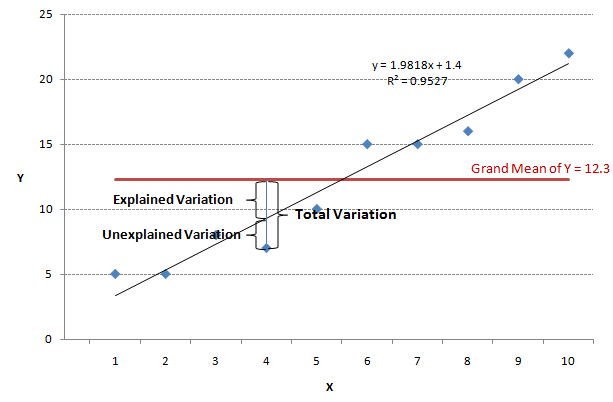
Sum of Squares Regression (SSR):

SSR quantifies the variation in Y that can be explained by the regression model. It measures how far the estimated regression line (ŷ) deviates from the horizontal "no relationship line", represented by the sample mean (ȳ). It is also called explained variation.

SSR = Σ(ŷ - ȳ)²

Sum of Squares Total (SST):

SST measures the total variation in the dependent variable (Y) without considering any regression model. It represents the variability in Y that is not explained by the model.

SST = SSR + SSE

Here, SSE = Sum of Squares Error (Unexplained Variation).

Interpretation of r²:

• 0 ≤ r² ≤ 1
• The higher the value of r², the better the fit of the regression to the data set
• Values of r² near one denote an extremely good fit of the regression to the data
• While values near zero denote an extremely poor fit.
• How “good” is regression model? Roughly:

0.8 ≤ r² ≤ 1 (STRONG)

0.5 ≤ r² < 0.8 (MEDIUM)

0 ≤ r² < 0.5 (WEAK)

Coefficient of Correlation (r):

• The coefficient of correlation, denoted as r, is a measure of the strength and direction of the linear relationship between two variables, typically X and Y. It represents the degree to which X and Y move together linearly.
• Formula: r is calculated as the square root of r².

r = √(r²)

• r ranges from -1 to 1. A positive value of r indicates a positive linear relationship, while a negative value of r indicates a negative linear relationship. The magnitude of r (how close it is to 1 or -1) tells you how strong the relationship is, with 1 or -1 indicating a perfect linear relationship.

Single Linear Regression Without Scikit-Learn:

import numpy as np
import pandas as pd
import matplotlib.pyplot as plt

# Create a sample dataset
data = {
    'Experience': [1, 2, 3, 4, 5, 6, 7, 8, 9, 10],
    'Salary': [45000, 50000, 60000, 65000, 70000, 75000, 85000, 90000, 95000, 100000]
}

df = pd.DataFrame(data)

# Features and target variable
X = np.array(df['Experience'])
y = np.array(df['Salary'])

# Calculate the coefficients using the given formula
n = len(X)
sum_x = np.sum(X)
sum_y = np.sum(y)
sum_xy = np.sum(X * y)
sum_x_squared = np.sum(X ** 2)

b1 = (n * sum_xy - sum_x * sum_y) / (n * sum_x_squared - sum_x ** 2)
b0 = np.mean(y) - b1 * np.mean(X)

print(f"Intercept (b0): {b0}")
print(f"Slope (b1): {b1}")

# Make predictions
y_pred = b0 + b1 * X

# Calculate R-squared
ss_total = np.sum((y - np.mean(y)) ** 2)
ss_residual = np.sum((y - y_pred) ** 2)
r_squared = 1 - (ss_residual / ss_total)
print(f"R-squared: {r_squared}")

# Coefficient of Correlation (r):
r = np.sqrt(r_squared)
print(f"r: {r}")

# Visualize the results
plt.scatter(X, y, color='blue')  # Scatter plot of the actual data
plt.plot(X, y_pred, color='red')  # Regression line
plt.xlabel('Years of Experience')
plt.ylabel('Salary')
plt.title('Salary vs. Experience')
plt.show()

# Intercept (b0): 39333.333333333336
# Slope (b1): 6212.121212121212
# R-squared: 0.9941333711825515
# r: 0.9970623707584955

Single Linear Regression With Scikit-Learn:

import pandas as pd
import numpy as np
from sklearn.model_selection import train_test_split
from sklearn.linear_model import LinearRegression
from sklearn.metrics import mean_squared_error, r2_score
import matplotlib.pyplot as plt

# Create a sample dataset
data = {
    'Experience': [1, 2, 3, 4, 5, 6, 7, 8, 9, 10, 11, 12],
    'Salary': [45000, 50000, 60000, 65000, 70000, 75000, 85000, 90000, 95000, 100000, 110000, 115000]
}

df = pd.DataFrame(data)

# Features and target variable
X = df[['Experience']]
y = df['Salary']

# Split the dataset into training and testing sets
X_train, X_test, y_train, y_test = train_test_split(X, y, test_size=0.2, random_state=42)

# Initialize the linear regression model
model = LinearRegression()

# Train the model
model.fit(X_train, y_train)

# Make predictions on the test set
y_pred = model.predict(X_test)

# Evaluate the model
mse = mean_squared_error(y_test, y_pred)
r2 = r2_score(y_test, y_pred)

# Coefficient of Correlation (r):
r = np.sqrt(r2)

print(f"Mean Squared Error: {mse}")
print(f"R-squared: {r2}")
print(f"r: {r}")

# Visualize the results
plt.scatter(X, y, color='blue')  # Scatter plot of the actual data
plt.plot(X, model.predict(X), color='red')  # Regression line
plt.xlabel('Years of Experience')
plt.ylabel('Salary')
plt.title('Salary vs. Experience')
plt.show()

# Mean Squared Error: 2383014.471042316
# R-squared: 0.9970820230966829
# r: 0.9985399456690167

Multiple Linear Regression

Multiple linear regression is used to estimate the relationship between two or more independent variables and one dependent variable.

For a multiple regression with p independent variables, the regression equation takes the form:

Y = β₀ + β₁X₁ + β₂X₂ + β₃X₃ + ... + βₚXₚ + ϵ

Multiple Linear Regression Model using Matrices:

Suppose that there are k independent variables X₁, X₂, …., Xₚ and p observations Y₁, Y₂, …., Yₚ, each of which can be expressed by the equation:

Y = β₀ + β₁X₁ + β₂X₂ + β₃X₃ + ... + βₚXₚ

The model essentially represents p equations describing how the response values are generated in the scientific process. Using matrix notation, we can write the following equation:

y = Xβ + ϵ

where:

• y is the vector of observed values.
• X is the matrix of feature values, where each row represents a data point and each column represents a feature.
• β is the vector of coefficients (including the intercept).
• ϵ is the error term.

Using the least squares method for the estimation of β, we can write the solution for the regression coefficients as:

Multiple Linear Regression Without Scikit-Learn:

import numpy as np
import pandas as pd

# Create a sample dataset
data = {
    'Experience': [1, 2, 3, 4, 5, 6, 7, 8, 9, 10],
    'Education': [1, 1, 1, 1, 2, 2, 2, 3, 3, 3],  # Dummy variable for education levels
    'Salary': [45000, 50000, 60000, 65000, 70000, 75000, 85000, 90000, 95000, 100000]
}

df = pd.DataFrame(data)

# Features and target variable
X = df[['Experience', 'Education']]
y = df['Salary']

# Step 2: Add a column of ones to X for the intercept term using pandas.concat()
intercept = pd.Series(np.ones(len(X)), name='Intercept')
X = pd.concat([intercept, X], axis=1)

# Step 3: Convert to numpy arrays
X = X.values
y = y.values.reshape(len(y), 1)

# Calculate the coefficients using the Normal Equation
beta = np.linalg.inv(X.T.dot(X)).dot(X.T).dot(y)

# Display the coefficients
print("Coefficients (including intercept):")
print(beta)

# Coefficients (including intercept):
# [[40000.        ]
#  [ 6666.66666667]
#  [-1666.66666667]]

# Make predictions
y_pred = X.dot(beta)

Multiple Linear Regression With Scikit-Learn:

import pandas as pd
import numpy as np
from sklearn.model_selection import train_test_split
from sklearn.linear_model import LinearRegression
from sklearn.metrics import mean_squared_error, r2_score

# Create a sample dataset
data = {
    'Experience': [1, 2, 3, 4, 5, 6, 7, 8, 9, 10, 11, 12],
    'Education': [1, 1, 1, 1, 2, 2, 2, 3, 3, 3, 3, 3],  # Dummy variable for education levels
    'Salary': [45000, 50000, 60000, 65000, 70000, 75000, 85000, 90000, 95000, 100000, 110000, 115000]
}

df = pd.DataFrame(data)

# Features and target variable
X = df[['Experience', 'Education']]
y = df['Salary']

# Split the dataset into training and testing sets
X_train, X_test, y_train, y_test = train_test_split(X, y, test_size=0.2, random_state=42)

# Initialize the linear regression model
model = LinearRegression()

# Train the model
model.fit(X_train, y_train)

# Make predictions on the test set
y_pred = model.predict(X_test)

# Evaluate the model
mse = mean_squared_error(y_test, y_pred)
r2 = r2_score(y_test, y_pred)
r = np.sqrt(r2)

print(f"Mean Squared Error: {mse}")
print(f"R-squared: {r2}")
print(f"r: {r}")

# Mean Squared Error: 1980391.5092262225
# R-squared: 0.9975750308050291
# r: 0.9987867794504637

Polynomial Regression

Polynomial regression is an extension of linear regression where the relationship between the independent variable X and the dependent variable y is modeled as an nth degree polynomial. While linear regression captures linear relationships, polynomial regression can capture more complex, non-linear relationships by adding polynomial terms to the model.

For a polynomial regression model of degree n, the model is:

where:

• β0, β1, …, βn are the coefficients of the polynomial terms,
• X is the independent variable,
• y is the dependent variable,
• ϵ is the error term.

Polynomial Regression (2nd Degree) Using Matrix Method:

In the case of a 2nd degree polynomial, the model can capture non-linear relationships by including quadratic terms.

The equation for a 2nd degree polynomial regression is:

In matrix form, the equation can be written as:

y = Xβ + ϵ

where:

• y is a vector of observed values,
• X is the design matrix containing the polynomial terms,
• β is a vector of coefficients,
• ϵ is a vector of errors.

For a 2nd degree polynomial, the design matrix X will include the intercept, the linear term, and the quadratic term:

The coefficients β can be calculated using the Normal Equation:

Polynomial Regression (2nd Degree) Without Scikit-learn:

import numpy as np
import pandas as pd
import matplotlib.pyplot as plt

# Sample data
data = {
    'X': [1, 2, 3, 4, 5],
    'y': [1, 4, 9, 16, 25]
}

df = pd.DataFrame(data)

# Features and target variable
X = df['X']
y = df['y']

# Create polynomial features manually (degree 2)
X_poly = pd.concat([pd.Series(1, index=df.index, name='Intercept'), X.rename('X'), (X**2).rename('X^2')], axis=1)

# Convert to numpy arrays
X_poly = X_poly.values
y = y.values.reshape(len(y), 1)

# Calculate the coefficients using the Normal Equation
beta = np.linalg.inv(X_poly.T.dot(X_poly)).dot(X_poly.T).dot(y)

# Display the coefficients
print("Coefficients (including intercept):")
print(beta)

# Coefficients (including intercept):
# [[-3.73034936e-14]
#  [ 7.01660952e-14]
#  [ 1.00000000e+00]]

# Make predictions
y_pred = X_poly.dot(beta)

# Visualize the results
plt.scatter(X, y, color='blue', label='Actual data')
plt.plot(X, y_pred, color='red', label='Polynomial regression fit')
plt.xlabel('X')
plt.ylabel('y')
plt.title('Polynomial Regression (Degree 2)')
plt.legend()
plt.show()

Polynomial Regression (2nd Degree) With Scikit-learn:

import numpy as np
import pandas as pd
import matplotlib.pyplot as plt
from sklearn.model_selection import train_test_split
from sklearn.preprocessing import PolynomialFeatures
from sklearn.linear_model import LinearRegression
from sklearn.metrics import r2_score

# Sample data
data = {
    'X': [1, 2, 3, 4, 5, 6, 7, 8, 9, 10],
    'y': [1, 4, 9, 16, 25, 36, 49, 64, 81, 100]
}

df = pd.DataFrame(data)

# Features and target variable
X = df[['X']]
y = df['y']

# Train-test split
X_train, X_test, y_train, y_test = train_test_split(X, y, test_size=0.2, random_state=42)

# Polynomial features (degree 2)
poly = PolynomialFeatures(degree=2)
X_train_poly = poly.fit_transform(X_train)
X_test_poly = poly.transform(X_test)

# Linear regression model
model = LinearRegression()
model.fit(X_train_poly, y_train)

# Make predictions
y_train_pred = model.predict(X_train_poly)
y_test_pred = model.predict(X_test_poly)

# Calculate R-squared
r_squared_test = r2_score(y_test, y_test_pred)
print(f"R-squared: {r_squared_test}")

# R-squared: 1.0

# Visualize the results
plt.scatter(X, y, color='blue', label='Actual data')
plt.plot(X, model.predict(poly.fit_transform(X)), color='red', label='Polynomial regression fit')
plt.xlabel('X')
plt.ylabel('y')
plt.title('Polynomial Regression (Degree 2)')
plt.legend()
plt.show()

Logistic Regression

Logistic Regression is a statistical method used for binary classification problems, where the outcome can be one of two possible classes. Despite its name, it is a classification algorithm, not a regression algorithm.

Key Concepts:

Binary Classification:

Logistic regression is used when the dependent variable is binary (e.g., yes/no, true/false, 0/1). For binary classification, the default threshold of a logistic regression model is 0.5, which means that data points with a higher probability than 0.5 will automatically be assigned a label of 1. This threshold value can be manually changed depending on our use case to achieve better results.

Logistic Function (Sigmoid Function):

• The logistic function is used to model the probability of the default class (e.g., class 1). The function is defined as:

• This function maps any real-valued number into a value between 0 and 1, which can be interpreted as a probability.

Odds and Log-Odds:

Odds:

Odds represent the ratio of the probability of an event occurring to the probability of it not occurring. If p is the probability of an event occurring, the odds are calculated as:

For example, if the probability of success is 0.8, the odds of success are 0.8 / 1−0.8 = 4. This means the event is 4 times more likely to occur than not.

Log-Odds (Logit):

Log-odds is the natural logarithm of the odds:

Log-odds can take any real value, from −∞ to +∞. When p=0.5, the log-odds is 0; when p>0.5, the log-odds is positive; and when p<0.5, the log-odds is negative.

Logistic Regression Model:

• The model predicts the log-odds of the probability of the default class as a linear combination of the input features.

• This can be rearranged to give the logistic regression equation:

Cost Function:

The cost function (or loss function) in logistic regression is typically the log-loss function, also known as cross-entropy loss. It measures how well the model’s predicted probabilities match the actual class labels.

Cost Function for Single Variable Logistic Regression

The cost function J(m,c) for logistic regression with a single feature is:

Gradient Descent for Single Variable Logistic Regression

To find the optimal values of m and c, we use gradient descent. Here's how you can update m and c:

1. Initialize Parameters: Start with initial guesses for m and c, such as zeros or small random values.

2. Compute Cost: Calculate the cost J(m,c) using the formula above with the current values of m and c.

3. Compute Gradients: The gradient of the cost function with respect to m and c is:

4. Update Parameters: Adjust the parameters m and c using the gradient descent update rules:

5. Repeat: Perform steps 2-4 iteratively until the cost function J(m,c) converges or a predetermined number of iterations is reached.

Example without Scikit-Learn:

import numpy as np
import pandas as pd

# Load data into a DataFrame
data = {
    'Exam': [34, 78, 50, 64, 84, 71, 58, 85, 52, 80],
    'Admitted': [0, 1, 0, 1, 1, 1, 0, 1, 0, 1]
}
df = pd.DataFrame(data)

# Feature and target variable
X = df['Exam'].values  # Feature
y = df['Admitted'].values  # Target

# Initialize parameters
initial_m = 0  # Slope (coefficient for feature)
initial_c = 0  # Intercept (bias)
learning_rate = 0.01
iterations = 100

# Logistic function
def sigmoid(z):
    return 1 / (1 + np.exp(-z))

# Cost function
def compute_cost(X, y, m, c):
    m_len = len(y)
    predictions = sigmoid(X * m + c)
    cost = - (1 / m_len) * np.sum(y * np.log(predictions + 1e-10) + (1 - y) * np.log(1 - predictions + 1e-10))
    return cost

# Gradient descent
def gradient_descent(X, y, initial_m, initial_c, learning_rate, iterations):
    m = initial_m
    c = initial_c
    m_len = len(y)
    
    for _ in range(iterations):
        predictions = sigmoid(X * m + c)
        dm = (1 / m_len) * np.sum((predictions - y) * X)
        dc = (1 / m_len) * np.sum(predictions - y)
        m -= learning_rate * dm
        c -= learning_rate * dc
        if _ % 10 == 0:  # Print cost every 100 iterations
            cost = compute_cost(X, y, m, c)
            print(f"Iteration {_}: Cost {cost}, m {m}, c {c}")
    
    return m, c

# Iteration 0: Cost 2.60133655757625, m 0.134, c 0.001
# Iteration 10: Cost 2.848303091809326, m 0.14697095883338093, c -0.00940155424386083
# Iteration 20: Cost 7.332758863309545, m 0.3802339282859193, c -0.016653060673761832
# Iteration 30: Cost 1.6060634611918247, m -0.03154284320208059, c -0.03340413607242968
# Iteration 40: Cost 3.6474612990548936, m 0.188847149356087, c -0.04089628680343251
# Iteration 50: Cost 1.428135996573944, m -0.02664153937132771, c -0.05477978970414606
# Iteration 60: Cost 0.7372009867978311, m -0.002344739926482372, c -0.0649032915576932
# Iteration 70: Cost 1.8351551181173589, m -0.0366997224083879, c -0.07611315549547003
# Iteration 80: Cost 7.337393219604362, m 0.3818343611545342, c -0.08044906392412234
# Iteration 90: Cost 4.887186418445125, m -0.10442179080555059, c -0.09831876558576817

# Train the model
m_final, c_final = gradient_descent(X, y, initial_m, initial_c, learning_rate, iterations)

print(f"Final parameters: m = {m_final}, c = {c_final}")

# Final parameters: m = -0.058886829620213216, c = -0.10727523723601864

# Predict function
def predict(X, m, c):
    return sigmoid(X * m + c) >= 0.5

# Test the model
predictions = predict(X, m_final, c_final)

Example with Scikit-Learn:

import pandas as pd
import numpy as np
from sklearn.linear_model import LogisticRegression
from sklearn.metrics import confusion_matrix, accuracy_score, precision_score, recall_score, f1_score
import matplotlib.pyplot as plt

# Load data into a DataFrame
data = {
    'Exam': [34, 78, 50, 64, 84, 71, 58, 85, 52, 80],
    'Admitted': [0, 1, 0, 1, 1, 1, 0, 1, 0, 1]
}
df = pd.DataFrame(data)

# Feature and target variable
X = df[['Exam']]  # Feature needs to be a 2D array
y = df['Admitted']

# Initialize and train the logistic regression model
model = LogisticRegression()
model.fit(X, y)

# Predict on the same data
predictions = model.predict(X)
probs = model.predict_proba(X)[:, 1]

# Confusion matrix
cm = confusion_matrix(y, predictions)
print(f"Confusion Matrix:\n{cm}")

# Accuracy
accuracy = accuracy_score(y, predictions)
print(f"Accuracy: {accuracy}")

# Precision
precision = precision_score(y, predictions)
print(f"Precision: {precision}")

# Recall
recall = recall_score(y, predictions)
print(f"Recall: {recall}")

# F1 Score
f1 = f1_score(y, predictions)
print(f"F1 Score: {f1}")

# Confusion Matrix:
# [[4 0]
#  [0 6]]
# Accuracy: 1.0
# Precision: 1.0
# Recall: 1.0
# F1 Score: 1.0

Classification Metrics

Confusion Matrix:

A confusion matrix is a summary of prediction results on a classification problem. The number of correct and incorrect predictions is summarized with count values and broken down by each class.

For a binary classification problem, the confusion matrix is a 2x2 table:

• True Positives (TP): The number of positive instances correctly classified.
• True Negatives (TN): The number of negative instances correctly classified.
• False Positives (FP): The number of negative instances incorrectly classified as positive.
• False Negatives (FN): The number of positive instances incorrectly classified as negative.

Example:

ID	Actual Sick	Predicted Sick	Outcome
1	1	1	TP
2	0	0	TN
3	0	0	TN
4	1	1	TP
5	0	0	TN
6	0	0	TN
7	1	0	FN
8	0	1	FP
9	0	0	TN
10	1	0	FN

Accuracy:

Accuracy is the ratio of correctly predicted instances to the total instances. It is a good measure when the classes are balanced.

Accuracy = TP+TN / TP+TN+FP+FN

Precision:

Precision (also called Positive Predictive Value) is the ratio of correctly predicted positive observations to the total predicted positives.

Precision = TP+FP / TP

Recall:

Recall (also called Sensitivity or True Positive Rate) is the ratio of correctly predicted positive observations to all observations in the actual class.

Recall = TP / TP+FN

F1 Score:

The F1 Score is the weighted average of Precision and Recall. It ranges from 0 to 1, and it is useful when you need to take both precision and recall into account.

F1 Score = (2 × Precision×Recall) / Precision+Recall

Example:

ID	Actual Sick	Predicted Sick	Outcome
1	1	1	TP
2	0	0	TN
3	0	0	TN
4	1	1	TP
5	0	0	TN
6	0	0	TN
7	1	0	FN
8	0	1	FP
9	0	0	TN
10	1	0	FN

Accuracy: Accuracy = 2+5 / 2+5+1+2 = 0.7

Precision: Precision = 2 / 2+1 = 0.667

Recall: Recall = 2 / 2+2 = 0.5

F1 Score: F1 Score = (2×0.667×0.5) / 0.667+0.5 = 0.571

ROC Curve:

The Receiver Operator Characteristic (ROC) curve is an evaluation metric for binary classification problems. It is a probability curve that plots the TPR against FPR at various threshold values and essentially separates the signal from the noise. The Area Under the Curve (AUC) is the measure of the ability of a classifier to distinguish between classes and is used as a summary of the ROC curve.

FPR = FP+TN / FP

Ina ROC curve, a higher X-axis value indicates a higher number of Flase positives than True negatives. While a higher T-axis value indicates a higher number of True positives than False negatives. So, the choice of the threshold depends on the ability to balance False positives and False negatives.

import numpy as np
import matplotlib.pyplot as plt
from sklearn.metrics import roc_curve, roc_auc_score

# Actual labels and predicted probabilities
y_true = [1, 0, 0, 1, 0, 0, 1, 0, 0, 1]
y_scores = [0.9, 0.1, 0.2, 0.8, 0.3, 0.2, 0.4, 0.7, 0.1, 0.3]

# Compute ROC curve
fpr, tpr, thresholds = roc_curve(y_true, y_scores)

# Compute AUC
auc = roc_auc_score(y_true, y_scores)

# Display thresholds
for i in range(len(thresholds)):
    print(f'Threshold: {thresholds[i]:.2f}, TPR: {tpr[i]:.2f}, FPR: {fpr[i]:.2f}')
    
# Threshold: 1.90, TPR: 0.00, FPR: 0.00
# Threshold: 0.90, TPR: 0.25, FPR: 0.00
# Threshold: 0.80, TPR: 0.50, FPR: 0.00
# Threshold: 0.70, TPR: 0.50, FPR: 0.17
# Threshold: 0.40, TPR: 0.75, FPR: 0.17
# Threshold: 0.30, TPR: 1.00, FPR: 0.33
# Threshold: 0.10, TPR: 1.00, FPR: 1.00

# Plot ROC curve
plt.figure()
plt.plot(fpr, tpr, label=f'ROC curve (area = {auc:.2f})')
plt.plot([0, 1], [0, 1], 'k--')  # Diagonal line
plt.xlim([0.0, 1.0])
plt.ylim([0.0, 1.0])
plt.xlabel('False Positive Rate')
plt.ylabel('True Positive Rate')
plt.title('Receiver Operating Characteristic (ROC) Curve')
plt.legend(loc="lower right")
plt.show()

Choosing the optimal threshold depends on the specific requirements of our application, such as the balance between True Positive Rate (TPR) and False Positive Rate (FPR). common method is to use the point on the ROC curve that is closest to the top-left corner (maximizing TPR while minimizing FPR) or to maximize some measure like Youden's J statistic (TPR - FPR).

1. Calculate TPR and FPR for each threshold:

• Threshold = 0.90: TPR = 0.25, FPR = 0.00
• Threshold = 0.80: TPR = 0.50, FPR = 0.00
• Threshold = 0.70: TPR = 0.50, FPR = 0.17
• Threshold = 0.40: TPR = 0.75, FPR = 0.17
• Threshold = 0.30: TPR = 1.00, FPR = 0.50
• Threshold = 0.20: TPR = 1.00, FPR = 0.67

2. Compute Youden's J statistic:

• Threshold = 0.90: Youden's J = 0.25 - 0.00 = 0.25
• Threshold = 0.80: Youden's J = 0.50 - 0.00 = 0.50
• Threshold = 0.70: Youden's J = 0.50 - 0.17 = 0.33
• Threshold = 0.40: Youden's J = 0.75 - 0.17 = 0.58
• Threshold = 0.30: Youden's J = 1.00 - 0.50 = 0.50
• Threshold = 0.20: Youden's J = 1.00 - 0.67 = 0.33

3. Select the threshold with the highest Youden's J:

• Optimal Threshold: 0.40 (Youden's J = 0.58)

K-Nearest Neighbors (KNN)

Classification:

K-Nearest Neighbors (KNN) classification is a simple and intuitive classification algorithm. It classifies a data point based on the majority class among its k-nearest neighbors.

Algorithm: Predicting Movie Genre

Dataset:

We have a small dataset of movies with their IMDb ratings, duration, and genre:

IMDb Rating	Duration	Genre
8.0	160	Action
6.2	170	Action
7.2	160	Comedy
8.2	155	Comedy

New Data Point:

We want to predict the genre of the "Barbie" movie with an IMDb rating of 7.4 and duration of 144 minutes.

Step 1: Calculate Distances

Calculate the Euclidean distance between the new movie and each movie in the dataset.

• Distance to (8.0, 160): 16.01
• Distance to (6.2, 170): 26.02
• Distance to (7.2, 160): 16.00
• Distance to (8.2, 155): 11.03

Step 2: Select Nearest Neighbors

Choose the k smallest distances. Let's use k = 3. K = {11.03, 16.00, 16.01}

Step 3: Majority Voting (Classification)

• Check the genres of the nearest neighbors:
  • Distance 11.03 corresponds to (8.2, 155) → Comedy
  • Distance 16.00 corresponds to (7.2, 160) → Comedy
  • Distance 16.01 corresponds to (8.0, 160) → Action
• Majority voting: {Comedy, Comedy, Action}
• The predicted genre for "Barbie" is Comedy.

Example without Scikit-Learn:

import pandas as pd
import numpy as np

# Creating the dataset
data = {
    'IMDb_Rating': [8.0, 6.2, 7.2, 8.2],
    'Duration': [160, 170, 160, 155],
    'Genre': ['Action', 'Action', 'Comedy', 'Comedy']
}
movies = pd.DataFrame(data)

# New movie data
new_movie = {'IMDb_Rating': 7.4, 'Duration': 144}
new_movie_df = pd.DataFrame([new_movie])

# Function to calculate Euclidean distance
def euclidean_distance(row1, row2):
    return np.sqrt((row1['IMDb_Rating'] - row2['IMDb_Rating'])**2 + (row1['Duration'] - row2['Duration'])**2)

# Calculate distances
movies['Distance'] = movies.apply(lambda row: euclidean_distance(row, new_movie_df.loc[0]), axis=1)

# Select k nearest neighbors
k = 3
nearest_neighbors = movies.nsmallest(k, 'Distance')

# Majority voting
predicted_genre = nearest_neighbors['Genre'].mode()[0]

print(f"The predicted genre for the movie 'Barbie' is: {predicted_genre}")

# The predicted genre for the movie 'Barbie' is: Comedy

Example with Scikit-Learn:

import pandas as pd
from sklearn.model_selection import train_test_split
from sklearn.neighbors import KNeighborsClassifier
from sklearn.metrics import confusion_matrix, accuracy_score, precision_score, recall_score, f1_score
import matplotlib.pyplot as plt

# Creating the dataset with more movies
data = {
    'IMDb_Rating': [8.0, 6.2, 7.2, 8.2, 7.5, 6.5, 7.8, 8.5, 6.8, 7.0],
    'Duration': [160, 170, 160, 155, 145, 180, 150, 140, 165, 175],
    'Genre': ['Action', 'Action', 'Comedy', 'Comedy', 'Comedy', 'Action', 'Comedy', 'Action', 'Action', 'Comedy']
}
movies = pd.DataFrame(data)

# Features and labels
X = movies[['IMDb_Rating', 'Duration']]
y = movies['Genre']

# Use train_test_split to split the data into training and testing sets with a test size of 30%.
X_train, X_test, y_train, y_test = train_test_split(X, y, test_size=0.3, random_state=42)

# KNN classifier
k = 2
knn = KNeighborsClassifier(n_neighbors=k)
knn.fit(X_train, y_train)

# Predict on the test set
y_pred = knn.predict(X_test)

print("Predicted genres:", y_pred)

# Performance metrics
# Confusion Matrix
cm = confusion_matrix(y_test, y_pred, labels=['Action', 'Comedy'])
print("Confusion Matrix:\n", cm)

# Accuracy
accuracy = accuracy_score(y_test, y_pred)
print("Accuracy:", accuracy)

# Precision
precision = precision_score(y_test, y_pred, average='weighted')
print("Precision:", precision)

# Recall
recall = recall_score(y_test, y_pred, average='weighted')
print("Recall:", recall)

# F1 Score
f1 = f1_score(y_test, y_pred, average='weighted')
print("F1 Score:", f1)

# Scatter plot
plt.figure(figsize=(10, 6))
# Plot training data
plt.scatter(X_train['IMDb_Rating'], X_train['Duration'], c=y_train.map({'Action': 'blue', 'Comedy': 'red'}), label='Training Data')
# Convert y_pred to a pandas Series
y_pred_series = pd.Series(y_pred, index=X_test.index)
# Plot test data with predicted labels
plt.scatter(X_test['IMDb_Rating'], X_test['Duration'], c=y_pred_series.map({'Action': 'cyan', 'Comedy': 'magenta'}), marker='x', label='Test Data (Predicted)')

plt.xlabel('IMDb Rating')
plt.ylabel('Duration')
plt.legend()
plt.title('KNN Classification of Movies')
plt.show()

# Predicted genres: ['Action' 'Comedy' 'Comedy']
# Confusion Matrix:
#  [[1 2]
#  [0 0]]
# Accuracy: 0.3333333333333333
# Precision: 1.0
# Recall: 0.3333333333333333
# F1 Score: 0.5

Regression:

K-Nearest Neighbors (KNN) is also used for regression tasks. In KNN regression, the target value is predicted based on the average of the target values of its k-nearest neighbors.

Algorithm: Predicting House Prices

Dataset:

We have a small dataset of houses with their size (in square feet), number of bedrooms, and price:

Size (sq ft)	Bedrooms	Price (in $1000s)
1500	3	300
1700	4	350
1600	3	320
1800	4	360

New Data Point:

We want to predict the price of a house with a size of 1650 sq ft and 3 bedrooms.

Step 1: Calculate Distances

Calculate the Euclidean distance between the new house and each house in the dataset.

• Distance to (1500, 3): 150
• Distance to (1700, 4): 50.01
• Distance to (1600, 3): 50
• Distance to (1800, 4): 150.01

Step 2: Select Nearest Neighbors

Choose the k smallest distances. Let's use k = 3.

K = {50, 50.01, 150}

Step 3: Average Target Values (Regression)

Check the prices of the nearest neighbors:

• Distance 50 corresponds to (1600, 3) → Price: $320k
• Distance 50.01 corresponds to (1700, 4) → Price: $350k
• Distance 150 corresponds to (1500, 3) → Price: $300k

Average the prices:

Predicted Price = (320 + 350 + 300) / 3 = 970 / 3 ≈ 323.3 (in $1000s)

import pandas as pd
from sklearn.neighbors import KNeighborsRegressor

# Dataset
data = {
    'Size (sq ft)': [1500, 1700, 1600, 1800],
    'Bedrooms': [3, 4, 3, 4],
    'Price (in $1000s)': [300, 350, 320, 360]
}
df = pd.DataFrame(data)

# Features and target
X = df[['Size (sq ft)', 'Bedrooms']]
y = df['Price (in $1000s)']

# New data point
new_house = pd.DataFrame({'Size (sq ft)': [1650], 'Bedrooms': [3]})

# Initialize KNN Regressor
knn_reg = KNeighborsRegressor(n_neighbors=3)

# Train the model
knn_reg.fit(X, y)

# Make prediction
predicted_price = knn_reg.predict(new_house)

print("Predicted price for the house:", predicted_price)

# Predicted price for the house: [323.33333333]

Decision Tree

Decision trees are a type of supervised learning algorithm that can be used for both classification and regression tasks. The goal of a decision tree is to create a model that predicts the value of a target variable by learning simple decision rules inferred from the data features. This model allows us to continuously split the dataset based on specific parameters until a final decision is made.

Decision Tree Terminology:

• Root Node: The topmost node in a decision tree.
• Internal Nodes: Nodes that split into more nodes.
• Leaf Nodes: Terminal nodes that do not split further.
• Branches: The connections between nodes.

Example 1 (Classification with Categorical Independent Variables):

Consider a dataset about whether a student will play a sport based on weather conditions:

Day	Weather	Temperature	Humidity	Wind	PlaySport
1	Sunny	Hot	High	Weak	No
2	Sunny	Hot	High	Strong	No
3	Overcast	Hot	High	Weak	Yes
4	Rain	Mild	High	Weak	Yes
5	Rain	Cool	Normal	Weak	Yes
6	Rain	Cool	Normal	Strong	No
7	Overcast	Cool	Normal	Strong	Yes
8	Sunny	Mild	High	Weak	No
9	Sunny	Cool	Normal	Weak	Yes
10	Rain	Mild	Normal	Weak	Yes
11	Sunny	Mild	Normal	Strong	Yes
12	Overcast	Mild	High	Strong	Yes
13	Overcast	Hot	Normal	Weak	Yes
14	Rain	Mild	High	Strong	No

Step 1: Calculate Entropy for the Target Variable

Entropy:

Entropy is a measure of uncertainty or randomness. In the context of decision trees, it helps us determine how a feature splits the data. The goal is to reduce entropy, or in other words, to make the data more homogeneous (less random).

• Target variable: Play Tennis (Yes/No)
• Total instances: 14

p(Yes) = 9/14

p(No) = 5/14

Entropy(Play Tennis) = - [p(Yes) * log2(p(Yes)) + p(No) * log2(p(No))]

= - [(9/14) * log2(9/14) + (5/14) * log2(5/14)]

≈ 0.940

Step 2: Calculate Information Gain for Each Attribute

We'll calculate the information gain for each attribute (Outlook, Temp, Humidity, Wind) to determine the best attribute to split the dataset.

Information Gain (IG) = Entropy(parent) - [Weighted Average * Entropy(children)]

Information Gain for Outlook

Sunny:

• p(Yes) = 2/5
• p(No) = 3/5
• Entropy(Sunny) = -[(2/5) * log2(2/5) + (3/5) * log2(3/5)] ≈ 0.971

Overcast:

• p(Yes) = 4/4 = 1
• p(No) = 0/4 = 0
• Entropy(Overcast) = 0

Rain:

• p(Yes) = 3/5
• p(No) = 2/5
• Entropy(Rain) = -[(3/5) * log2(3/5) + (2/5) * log2(2/5)] ≈ 0.971

Weighted Average Entropy:

• (5/14) * 0.971 + (4/14) * 0 + (5/14) * 0.971 ≈ 0.693

Information Gain:

• 0.940 - 0.693 ≈ 0.247

Hence,

Information Gain for Temp: 0.0289

Information Gain for Humidity: 0.1516

Information Gain for Wind: 0.0478

Step 3: Choose the Best Attribute

Select the attribute with the highest information gain as the root node of the decision tree. In this case, Outlook has the highest information gain.

Step 4: Split the Dataset

Split the dataset based on the chosen attribute (Outlook) and repeat steps 1-3 for each subset.

Now, for sunny Dataset:

Day	Temperature	Humidity	Wind	PlaySport
1	Hot	High	Weak	No
2	Hot	High	Strong	No
8	Mild	High	Weak	No
9	Cool	Normal	Weak	Yes
11	Mild	Normal	Strong	Yes

Information Gain for Temp: 0.570

Information Gain for Humidity: 0.97

Information Gain for Wind: 0.0192

Step 5: Build the Decision Tree

Continue splitting the dataset until you reach a pure node (all instances belong to the same class) or a predefined stopping criterion.

import numpy as np
import pandas as pd
from sklearn.tree import DecisionTreeClassifier
import matplotlib.pyplot as plt

# Create a sample dataset
data = {
    'Weather': ['Sunny', 'Sunny', 'Overcast', 'Rain', 'Rain', 'Rain', 'Overcast', 'Sunny', 'Sunny', 'Rain', 'Sunny', 'Overcast', 'Overcast', 'Rain'],
    'Temperature': ['Hot', 'Hot', 'Hot', 'Mild', 'Cool', 'Cool', 'Cool', 'Mild', 'Cool', 'Mild', 'Mild', 'Mild', 'Hot', 'Mild'],
    'Humidity': ['High', 'High', 'High', 'High', 'Normal', 'Normal', 'Normal', 'High', 'Normal', 'Normal', 'Normal', 'High', 'Normal', 'High'],
    'Wind': ['Weak', 'Strong', 'Weak', 'Weak', 'Weak', 'Strong', 'Strong', 'Weak', 'Weak', 'Weak', 'Strong', 'Strong', 'Weak', 'Strong'],
    'PlaySport': ['No', 'No', 'Yes', 'Yes', 'Yes', 'No', 'Yes', 'No', 'Yes', 'Yes', 'Yes', 'Yes', 'Yes', 'No']
}

df = pd.DataFrame(data)

# Convert categorical features to numerical
df_encoded = pd.get_dummies(df.drop('PlaySport', axis=1))
y = df['PlaySport'].map({'No': 0, 'Yes': 1})

# Train the decision tree classifier
clf = DecisionTreeClassifier(criterion='entropy')
clf.fit(df_encoded, y)

# Predict the target values
predictions = clf.predict(df_encoded)

# Create a simple line plot for predicted data
plt.figure(figsize=(10, 6))
plt.plot(range(len(y)), y, label='Actual', marker='o')
plt.plot(range(len(y)), predictions, label='Predicted', marker='x', linestyle='--')
plt.xlabel('Sample Index')
plt.ylabel('PlaySport')
plt.title('Actual vs Predicted Values')
plt.legend()
plt.show()

Example 2 (Regression with Categorical Independent Variables):

Consider a dataset:

Day	Weather	Temperature	Humidity	Wind	Golf Players
1	Sunny	Hot	High	Weak	25
2	Sunny	Hot	High	Strong	30
3	Overcast	Hot	High	Weak	46
4	Rain	Mild	High	Weak	45
5	Rain	Cool	Normal	Weak	52
6	Rain	Cool	Normal	Strong	23
7	Overcast	Cool	Normal	Strong	43
8	Sunny	Mild	High	Weak	35
9	Sunny	Cool	Normal	Weak	38
10	Rain	Mild	Normal	Weak	46
11	Sunny	Mild	Normal	Strong	48
12	Overcast	Mild	High	Strong	52
13	Overcast	Hot	Normal	Weak	44
14	Rain	Mild	High	Strong	30

Step 1: Calculate global standard deviation of the Target Variable:

We start by calculating the standard deviation of the Golf Players across all instances.

Step 2: Calculate the weighted standard deviation for each potential split (feature) and compute the standard deviation reduction for each split:

We will calculate the standard deviation reduction for each feature (Outlook, Temp, Humidity, Wind).

For Outlook:

Sunny:

Overcast:

Rain:

Weighted Standard Deviation for Outlook:

Standard Deviation Reduction for Outlook:

For Other Features:

Feature	STD Reduction
Temperature	0.47
Humidity	0.27
Wind	0.29

Step 3: Choose the best split (the one with the highest standard deviation reduction):

The best feature to split on is Outlook with a standard deviation reduction of 0.89.

As there are less than 5 training examples in the Overcast branch so we take the average value 46, and we stop there.

Now, repeat the process for the other resulting subsets until stopping criteria are met.

import pandas as pd
import numpy as np
from sklearn.tree import DecisionTreeRegressor
import matplotlib.pyplot as plt

# Sample dataset
data = {
    'Outlook': ['Sunny', 'Sunny', 'Overcast', 'Rain', 'Rain', 'Rain', 'Overcast', 'Sunny', 'Sunny', 'Rain', 'Sunny', 'Overcast', 'Overcast', 'Rain'],
    'Temp': ['Hot', 'Hot', 'Hot', 'Mild', 'Cool', 'Cool', 'Cool', 'Mild', 'Cool', 'Mild', 'Mild', 'Mild', 'Hot', 'Mild'],
    'Humidity': ['High', 'High', 'High', 'High', 'Normal', 'Normal', 'Normal', 'High', 'Normal', 'Normal', 'Normal', 'High', 'Normal', 'High'],
    'Wind': ['Weak', 'Strong', 'Weak', 'Weak', 'Weak', 'Strong', 'Strong', 'Weak', 'Weak', 'Weak', 'Strong', 'Strong', 'Weak', 'Strong'],
    'Golf_Players': [25, 30, 46, 45, 52, 23, 43, 35, 38, 46, 48, 52, 44, 30]
}

df = pd.DataFrame(data)

# Encode categorical features
df_encoded = pd.get_dummies(df[['Outlook', 'Temp', 'Humidity', 'Wind']])
X = df_encoded.values
y = df['Golf_Players'].values

# Train Decision Tree Regressor
regressor = DecisionTreeRegressor()
regressor.fit(X, y)

# Predicting the values
predictions = regressor.predict(X)

# Plotting the results
plt.figure(figsize=(10, 6))
plt.plot(range(len(y)), y, label='Actual', marker='o')
plt.plot(range(len(y)), predictions, label='Predicted', marker='x', linestyle='--')
plt.xlabel('Sample Index')
plt.ylabel('Golf Players')
plt.title('Actual vs Predicted Golf Players')
plt.legend()
plt.show()

Example 3 (Classification with Continuous Independent Variables):

Consider a dataset:

Annual Income	Label
60	No
70	No
75	Yes
85	Yes
90	Yes
100	No
120	No
125	No
220	No

Step 1: Select Split points based on the given data set:

For a continuous attribute, potential split points are typically chosen at the midpoints between consecutive values. This ensures that all potential splits are considered. For the given dataset, the midpoints are:

• (60 + 70) / 2 = 65
• (70 + 75) / 2 = 72.5
• (75 + 85) / 2 = 80
• (85 + 90) / 2 = 87.5
• (90 + 95) / 2 = 92.5
• (95 + 100) / 2 = 97.5
• (100 + 120) / 2 = 110
• (120 + 125) / 2 = 122.5
• (125 + 220) / 2 = 172.5

We will select 80 and 97.5.

Step 2: Compute Gini Index for Different Split Points to find Optimal Split Point:

The Gini index for a split is calculated using the formula:

We'll compute the Gini index for different split points to find the optimal split.

Calculation for Split at 80

1. Groups after Split:

• Left Group: [60, 70, 75] (All 'No')
• Right Group: [85, 90, 95, 100, 120, 125, 220] (3 'Yes', 4 'No')

2. Gini Index for Left Group:

3. Gini Index for Right Group:

4. Weighted Gini Index:

Calculation for Split at 97.5

1. Groups after Split:

• Left Group: [60, 70, 75, 85, 90, 95] (3 'No', 3 'Yes')
• Right Group: [100, 120, 125, 220] (All 'No')

2. Gini Index for Left Group:

3. Gini Index for Right Group:

4. Weighted Gini Index:

Comparison of Gini Indices

• Split at 80: Gini Index = 0.3429
• Split at 97.5: Gini Index = 0.3

The optimal split point is at 97.5 since it has a lower Gini index.

import numpy as np
import pandas as pd
from sklearn.tree import DecisionTreeClassifier
import matplotlib.pyplot as plt

# Create a sample dataset
data = {
    'Annual Income': [60, 70, 75, 85, 90, 95, 100, 120, 125, 220],
    'Label': ['No', 'No', 'No', 'Yes', 'Yes', 'Yes', 'No', 'No', 'No', 'No']
}

df = pd.DataFrame(data)

# Encode the labels
df['Label'] = df['Label'].map({'No': 0, 'Yes': 1})

# Define features and target
X = df[['Annual Income']]
y = df['Label']

# Initialize and train the decision tree classifier
clf = DecisionTreeClassifier(criterion='gini')
clf.fit(X, y)

Note: We can also use the entropy method instead of the Gini index to evaluate the quality of a split in a decision tree. The split with the lowest weighted entropy indicates the best split point.

Random Forest

A Random Forest is an ensemble learning method that combines multiple decision trees to improve classification and regression performance. Here’s a brief overview of how it works:

Ensemble Learning:

Instead of relying on a single decision tree, a Random Forest builds multiple trees and aggregates their predictions. This helps in reducing overfitting and improving accuracy.

Bootstrapping:

Random Forest uses a technique called bootstrapping to create multiple subsets of the training data by sampling with replacement. Each decision tree is trained on a different subset of the data.

Example:

• Original Dataset:

Email Length	Has Attachments	Spam
100	Yes	Yes
150	No	No
200	Yes	Yes
250	No	No
300	Yes	Yes
350	No	No
400	Yes	Yes
450	No	No

• Bootstrapped Subsets: Random Forest might create several bootstrapped samples. For instance, one subset might look like:

Email Length	Has Attachments	Spam
100	Yes	Yes
200	Yes	Yes
300	Yes	Yes
100	Yes	Yes

Another subset might look like:

Email Length	Has Attachments	Spam
150	No	No
250	No	No
350	No	No
250	No	No

Each decision tree is trained on one of these subsets, leading to diversity among the trees.

Feature Randomness:

When splitting nodes, Random Forest considers a random subset of features rather than all features. This introduces diversity among the trees and helps in making the ensemble more robust.

Example:

Feature Subsets: Suppose we have two features: Email Length and Has Attachments. For a particular split, a decision tree might only consider one of these features (e.g., Email Length) to make a decision at a node, while another tree might consider the other feature (e.g., Has Attachments) or a different combination.

This randomness ensures that the trees are not overly correlated, leading to a more robust ensemble.

Voting/Averaging:

For classification, Random Forest uses majority voting (the class that gets the most votes is chosen). For regression, it averages the predictions of the individual trees.

Example:

• Classification Voting: Suppose we have 10 trees in our Random Forest. For an unseen email, each tree makes a classification (e.g., Spam or Not Spam). If 7 out of 10 trees classify the email as Spam, then the Random Forest will classify the email as Spam.
• Regression Averaging: If you were using Random Forest for regression, you would average the predictions from all the trees. For example, if individual trees predict values of 5, 6, 5, 7, and 6, the Random Forest would predict the average of these values.

Random Forest classifier using scikit-learn:

import numpy as np
from sklearn.model_selection import train_test_split
from sklearn.ensemble import RandomForestClassifier
from sklearn.datasets import load_iris

# Load a sample dataset (Iris dataset)
data = load_iris()
X = data.data
y = data.target

# Split the dataset into training and test sets
X_train, X_test, y_train, y_test = train_test_split(X, y, test_size=0.3, random_state=42)

# Initialize the Random Forest Classifier
rf_clf = RandomForestClassifier(n_estimators=100, random_state=42)

# Train the classifier
rf_clf.fit(X_train, y_train)

# Make predictions
y_pred = rf_clf.predict(X_test)

Unsupervised Learning

In unsupervised learning, the algorithm is given data without explicit instructions on what to do with it. The goal is to explore the structure of the data and extract meaningful information without specific guidance.

K-Means Clustering

K-Means Clustering is one of the most popular unsupervised learning algorithms. It partitions the data into K clusters, where each data point belongs to the cluster with the nearest mean. The algorithm aims to minimize the variance within each cluster.

Algorithm:

Data:

Individual	Variable 1	Variable 2
1	1.0	1.0
2	1.5	2.0
3	3.0	4.0
4	5.0	7.0
5	3.5	5.0
6	4.5	5.0
7	3.5	4.5

Step 1: Choose K initial centroids (points representing cluster centers):

Randomly we choose following two centroids (K = 2) for two clusters. In this case the 2 centroids are:

m1 = (1.0, 1.0) and m2 = (5.0, 7.0)

Step 2: Assign each data point to the nearest centroid, forming K clusters:

For this we have to find the distance of each data point by using formulas like Euclidean or Manhattan.

Euclidean:

Manhattan:

Individual	Variable 1	Variable 2	Distance from Centroid 1	Distance from Centroid 2
1	1.0	1.0	0	7.21
2	1.5	2.0	1.12	6.10
3	3.0	4.0	3.61	3.61
4	5.0	7.0	7.21	0
5	3.5	5.0	4.72	2.5
6	4.5	5.0	5.31	2.06
7	3.5	4.5	4.30	2.92

Thus, we obtain two clusters containing:

{1, 2, 3} and {4, 5, 6, 7}

Step 3: Recalculate the centroids as the mean of all points in the cluster:

m1 = (1/3 (1.0 + 1.5 + 3.0), 1/3 (1.0 + 2.0 + 4.0)) = (1.83, 2.33)

m2 = (1/4 (5.0 + 3.5 + 4.5, 3.5), 1/4 (7.0 + 5.0 + 5.0, 4.5)) = (4.12, 5.38)

Step 4: Repeat until there is no change in the cluster:

Individual	Variable 1	Variable 2	Distance from Centroid 1	Distance from Centroid 2
1	1.0	1.0	1.57	7.21
2	1.5	2.0	0.47	6.10
3	3.0	4.0	2.04	1.78
4	5.0	7.0	5.64	1.84
5	3.5	5.0	3.15	0.73
6	4.5	5.0	3.78	0.54
7	3.5	4.5	2.74	1.08

New Clusters: {1, 2} and {3, 4, 5, 6, 7}

New Centroids: m1 = (1.25, 1.5) and m2 = (3.9, 5.1)

Individual	Variable 1	Variable 2	Distance from Centroid 1	Distance from Centroid 2
1	1.0	1.0	0.58	5.02
2	1.5	2.0	0.58	3.92
3	3.0	4.0	3.05	1.42
4	5.0	7.0	6.66	2.20
5	3.5	5.0	4.18	0.41
6	4.5	5.0	4.78	0.61
7	3.5	4.5	3.75	0.72

Final 2 Clusters: {1, 2} and {3, 4, 5, 6, 7}

K-Means Clustering Without Sk-Learn:

import numpy as np

# Dataset
X = np.array([
    [1.0, 1.0],
    [1.5, 2.0],
    [3.0, 4.0],
    [5.0, 7.0],
    [3.5, 5.0],
    [4.5, 5.0],
    [3.5, 4.5]
])

# Parameters
K = 2  # number of clusters
max_iters = 100  # maximum number of iterations

# Initialize centroids randomly
np.random.seed(42)  # for reproducibility
centroids = X[np.random.choice(X.shape[0], K, replace=False)]

# Function to calculate Euclidean distance
def euclidean_distance(a, b):
    return np.sqrt(np.sum((a - b) ** 2))

# K-Means algorithm
for _ in range(max_iters):
    # Assign clusters
    clusters = [[] for _ in range(K)]
    for x in X:
        distances = [euclidean_distance(x, centroid) for centroid in centroids]
        cluster = np.argmin(distances)
        clusters[cluster].append(x)

    # Calculate new centroids
    new_centroids = np.array([np.mean(cluster, axis=0) for cluster in clusters])

    # Check for convergence
    if np.all(centroids == new_centroids):
        break
    centroids = new_centroids

# Print results
print("Centroids:")
print(centroids)

print("Clusters:")
for i, cluster in enumerate(clusters):
    print(f"Cluster {i+1}: {cluster}")
    
# Centroids:
# [[1.25 1.5 ]
#  [3.9  5.1 ]]
# Clusters:
# Cluster 1: [array([1., 1.]), array([1.5, 2. ])]
# Cluster 2: [array([3., 4.]), array([5., 7.]), array([3.5, 5. ]), array([4.5, 5. ]), array([3.5, 4.5])]

K-Means Clustering With Sk-Learn:

import numpy as np
from sklearn.cluster import KMeans
import pandas as pd

# Dataset
data = {
    'Individual': [1, 2, 3, 4, 5, 6, 7],
    'Variable 1': [1.0, 1.5, 3.0, 5.0, 3.5, 4.5, 3.5],
    'Variable 2': [1.0, 2.0, 4.0, 7.0, 5.0, 5.0, 4.5]
}
df = pd.DataFrame(data)
X = df[['Variable 1', 'Variable 2']]

# K-Means algorithm
kmeans = KMeans(n_clusters=2, random_state=42)
kmeans.fit(X)

# Get the centroids and labels
centroids = kmeans.cluster_centers_
labels = kmeans.labels_

# Print results
print("Centroids:")
print(centroids)

print("Labels:")
print(labels)

# Add cluster labels to the DataFrame
df['Cluster'] = labels
print("Clustered Data:")
print(df)

# Centroids:
# [[3.9  5.1 ]
#  [1.25 1.5 ]]
# Labels:
# [1 1 0 0 0 0 0]
# Clustered Data:
#    Individual  Variable 1  Variable 2  Cluster
# 0           1         1.0         1.0        1
# 1           2         1.5         2.0        1
# 2           3         3.0         4.0        0
# 3           4         5.0         7.0        0
# 4           5         3.5         5.0        0
# 5           6         4.5         5.0        0
# 6           7         3.5         4.5        0

Feature Subset Selection

Dimensionality Reduction:

• Definition: Dimensionality Reduction is the process of reducing the number of features (dimensions) in a dataset while retaining its essential information.
• Objective: Overcome the "curse of dimensionality", improve model efficiency, and enhance interpretability.
• Data preprocessing is an important part for effective machine learning.
• Dimensionality reduction is an effective approach to downsizing data.

Why Dimensionality Reduction?

• Curse of Dimensionality reduction: As the number of features decreases, the data becomes more accurate, and computational complexity decreases.
• Noise Removal: Some features may be noisy, leading to overfitting. So noise removal provides more accuracy in data.
• Data compression: Efficient storage and retrieval.
• Visualization: Projection of high-dimensional data onto 2D or 3D.
• Reduces training time in machine learning.

Techniques:

• Feature Selection: Choosing a subset of relevant features while discarding irrelevant or redundant ones (Only a subset of the original features are selected).
• Feature Extraction/Reduction: Feature Extraction/Reduction refers to the process of transforming or combining original features to create a more compact and representative set of features in a dataset.

Feature Selection

Feature or Variable Selection refers to the process of selecting features that are used in predicting the target or output.

The purpose of Feature Selection is to select the features that contribute the most to output prediction.

Methods:

• Filter Methods
• Wrapper Methods

Filter Methods:

• Definition: The Filter Methods involve selecting features based on their various statistical scores with the output column.
• The filter method ranks each feature based on some uni-variate metric and then selects the highest-ranking features. We identify and retain the most relevant features based on statistical measures or predefined criteria.
• The selection of features is independent of any Machine Learning algorithm.

• Rules:
• The more the features are correlated with the output column or the column to be predicted, the better the performance of the model.
• Features should be least correlated with each other. If some of the input features are correlated with some additional input features, this situation is known as Multicollinearity. It is recommended to get rid of such a situation for better performance of the model.

• Filter Selection Select independent features with:

• No constant variables
• No duplicate rows
• High correlation with the target variable
• Low correlation with another independent variable
• Higher information gain or mutual information of the independent variable

Common Filter Methods:

1. Removing features with low variance (Low variance filter):

Definition: The Low Variance Filter is a feature selection method that focuses on identifying and eliminating features with minimal variance across the dataset. Features with low variance often carry limited information and may not contribute significantly to the modeling process.

Key Components:

Variance:

• Measures the spread or variability of values within a feature.
• High variance indicates a wide range of values, while low variance suggests a more constant or uniform feature.

Threshold:

• A predetermined threshold is set to determine the acceptable level of variance.
• Features with variance below the threshold are considered low-variance features.

Steps:

To remove features with low variance from our dataset, follow these steps:

1. Remove features with zero variance (constants).
2. Normalize the data and compute the variance for each feature.
3. Choose a threshold value that defines the minimum acceptable variance.
4. Identify and remove features with variance below the selected threshold.

ID	season	holiday	workingday	weather	f5	temp	atemp	humidity	windspeed	count
AB101	1	0	0	1	7	9.84	14.395	81	0.0000	16
AB102	1	0	0	1	7	9.02	13.635	80	0.0000	40
AB103	1	0	0	1	7	9.02	13.635	80	0.0000	32
AB104	1	0	0	1	7	9.84	14.395	75	0.0000	13
AB105	1	0	0	1	7	9.84	14.395	75	0.0000	1
AB106	1	0	0	2	7	9.84	12.880	75	6.0032	1
AB107	1	0	0	1	7	9.02	13.635	80	0.0000	2
AB108	1	0	0	2	7	9.02	12.880	86	0.0000	3
AB109	1	0	0	1	7	9.84	14.395	75	0.0000	8
AB110	1	0	0	1	7	13.12	17.425	76	0.0000	14

import pandas as pd
from sklearn.preprocessing import StandardScaler

# Create the DataFrame
data = {
    'ID': ['AB101', 'AB102', 'AB103', 'AB104', 'AB105', 'AB106', 'AB107', 'AB108', 'AB109', 'AB110'],
    'season': [1, 1, 1, 1, 1, 1, 1, 1, 1, 1],
    'holiday': [0, 0, 0, 0, 0, 0, 0, 0, 0, 0],
    'workingday': [0, 0, 0, 0, 0, 0, 0, 0, 0, 0],
    'weather': [1, 1, 1, 1, 1, 2, 1, 2, 1, 1],
    'f5': [7, 7, 7, 7, 7, 7, 7, 7, 7, 7],
    'temp': [9.84, 9.02, 9.02, 9.84, 9.84, 9.84, 9.02, 9.02, 9.84, 13.12],
    'atemp': [14.395, 13.635, 13.635, 14.395, 14.395, 12.880, 13.635, 12.880, 14.395, 17.425],
    'humidity': [81, 80, 80, 75, 75, 75, 80, 86, 75, 76],
    'windspeed': [0.0000, 0.0000, 0.0000, 0.0000, 0.0000, 6.0032, 0.0000, 0.0000, 0.0000, 0.0000],
    'count': [16, 40, 32, 13, 1, 1, 2, 3, 8, 14]
}

df = pd.DataFrame(data)

# Drop the ID column as it is not a feature
df = df.drop(columns=['ID'])

# Step 1: Remove features with zero variance (constants)
df = df.loc[:, df.var() != 0]

# Step 2: Normalize the data
scaler = StandardScaler()
df_normalized = pd.DataFrame(scaler.fit_transform(df), columns=df.columns)

# Step 3: Compute the variance for each feature
variance = df_normalized.var()

print(variance)

# weather      1.111
# temp         1.111
# atemp        1.111
# humidity     1.111
# windspeed    1.111
# count        1.111

# Choose a threshold (e.g., 10% of the maximum variance)
threshold = 0.1 * variance.max()

# Step 4: Identify and remove low-variance features
low_variance_features = variance[variance < threshold].index
df_reduced = df.drop(columns=low_variance_features)

print("Remaining features:")
print(df_reduced.head())

# Remaining features:
#    weather  temp   atemp  humidity  windspeed  count
# 0        1  9.84  14.395        81        0.0     16
# 1        1  9.02  13.635        80        0.0     40
# 2        1  9.02  13.635        80        0.0     32
# 3        1  9.84  14.395        75        0.0     13
# 4        1  9.84  14.395        75        0.0      1

2. Pearson's Correlation Coefficient:

Definition: Pearson's Correlation Coefficient, often denoted as r, is a statistical measure that quantifies the strength and direction of a linear relationship between two continuous variables.

Objective: To determine the degree of linear association between two variables, with values ranging from -1 (perfect negative correlation) to 1 (perfect positive correlation), and 0 indicating no linear correlation.

Formula:

The Pearson correlation coefficient is calculated using the following formula:

Example: A researcher in a scientific foundation wished to evaluate the relation between annuals salaries of mathematicians (Y, in thousand dollars) and an index of work quality (X1), number of years of experience (X2), and an index of publication success (X3).

Index of Work Quality (X1)	Number of Years of Experience (X2)	Index of Publication Success (X3)	Annual Salaries (in thousand dollars) Y
3.5	9	6.1	33.2
5.1	18	7.4	38.7
6	13	5.9	37.5
3.1	5	5.8	30.1
4.5	25	5	38.2

Heat Map:

A Heat Map is a graphical representation that visualizes the strength and direction of relationships between multiple variables, often using color gradients.

• Calculate Pearson's correlation coefficient for all pairs of variables in the dataset.
• Represent the correlation matrix as a heat map, where each cell color corresponds to the correlation value.

• Handling Multicollinearity:
• Address multicollinearity issues, especially when features are highly correlated.
• Choose features with the least redundancy.

3. Mutual Information (Information Gain):

Definition: Mutual Information measures the amount of information obtained about one variable through the observation of another variable. In the context of feature selection, it quantifies the degree of dependence between a feature and the target variable.

The feature having the most information is considered important by the algorithm and is used for training the model.

The effort is to reduce the entropy and maximize the information gain.

Entropy:

• A measure of uncertainty or randomness in a variable.
• High entropy indicates greater uncertainty.
• Information gain uses entropy to make decisions. If the entropy is less, information will be more.

Formula:

The Mutual Information between two variables X and Y is calculated using the following formula:

IG (X|Y) = E(S) - E (X|Y)

Example:

Suppose we have the following given data set:

Continents	movieSuccess
Australia	T
Australia	F
Australia	T
Europe	T
Europe	F
Europe	F
Asia	F
Asia	F
Europe	T
Australia	T

To find the information gain using entropy, we'll go through the following steps:

Step 1: Calculate the Entropy of the Entire Dataset (S)

Entropy E(S) is given by the formula:

For the given dataset:

• Total instances (S): 10
• Success (T): 5
• Failure (F): 5

p(T) = 5/10 = 0.5

p(F) = 5/10 = 0.5

E(S) = - (0.5 log_2 0.5 + 0.5 log_2 0.5)

E(S) = - (0.5 * -1 + 0.5 * -1)

E(S) = 1

Step 2: Calculate the Entropy for Each Subset After the Split

Australia:

• Total instances: 4
• Success (T): 3
• Failure (F): 1

p(T) = 3/4 = 0.75

p(F) = 3/4 = 0.25

E(Australia) = - (0.75 log_2 0.75 + 0.25 log_2 0.25)

E(Australia) = - (0.75 * -0.415 + 0.25 * -2)

E(Australia) = - (-0.31125 - 0.5)

E(Australia) = 0.81125

Europe:

• Total instances: 4
• Success (T): 2
• Failure (F): 2

p(T) = 2/4 = 0.5

p(F) = 2/4 = 0.5

E(Europe) = - (0.5 log_2 0.5 + 0.5 log_2 0.5)

E(Europe) = - (0.5 * -1 + 0.5 * -1)

E(Europe) = 1

Asia:

• Total instances: 2
• Success (T): 0
• Failure (F): 2

p(T) = 0/2 = 0

p(F) = 2/2 = 1

E(Asia) = - (0 log_2 0 + 1 log_2 1)

E(Asia) = 0

Step 3: Calculate the Weighted Sum of the Entropies of the Subsets

E(X|Y) = 4/10 * E(Australia) + 4/10 * E(Europe) + 2/10 * E(Asia)

E(X|Y) = 0.7245

Step 4: Calculate the Information Gain

IG(X|Y) = E(S) - E(X|Y)

IG(X|Y) = 1 - 0.7245

IG(X|Y) = 0.2755

Thus, the information gain from splitting the dataset based on continents is 0.2755.

Advantages of Filter methods:

• Filter methods are model agnostic(compatible)
• Rely entirely on features in the data set
• Computationally very fast
• Based on different statistical methods

Disadvantages of Filter methods:

• The filter method looks at individual features for identifying it’s relative importance. A feature may not be useful on its own but may be an important influencer when combined with other features. Filter methods may miss such features.
• One thing that should be kept in mind is that the filter method does not correctly remove multicollinearity. So, you must deal with the multicollinearity of features as well before training models for your data.

Wrapper Methods:

Definition: In Wrapper Methods the problem of Feature Selection is reduced to a search problem.

A model is built using a set of features and its accuracy is recorded.

Based on the accuracy, more features are added or removed, and the process is repeated.

Common Wrapper Methods:

1. Forward Selection:

• Forward Selection is an iterative method.
• In this method, we start with one feature and we keep on adding features until no improvement in the model is observed.
• The search is stopped after a pre-set criteria is met.
• This is a greedy approach because it always targets the features in a forward fashion, which gives a boost to the performance.
• If the number of features are large, it can be computationally expensive.

2. Backward Elimination:

• This process is the opposite of the Forward Selection Method.
• It starts initially with all the features and keeps on removing features until no improvement is observed.

Forward Feature Selection:

Forward Feature Selection is a stepwise process for selecting important features for a predictive model. It begins with an empty model and iteratively adds features that improve the model's performance the most. Here's how you can perform forward feature selection:

• Select the Best Single Feature: Add each feature to the model individually and select the one that improves the model's performance the most.
• Add the Next Best Feature: Add each of the remaining features to the current model (one at a time) and select the one that provides the best performance improvement.
• Repeat the Process: Continue adding features one by one, selecting the one that improves the model the most each time, until adding more features does not significantly improve the model's performance or a stopping criterion is met.
• Final Model: The process stops when no additional features improve the model significantly or when a predefined number of features is reached.

Example:

Let's use the given dataset to perform forward feature selection to predict the Fitness Level.

Initial Dataset:

ID	Calories Burnt	Gender	Plays Sport?	Fitness Level
1	121	M	Yes	Fit
2	230	M	No	Fit
3	342	F	No	Unfit
4	70	M	Yes	Fit
5	278	F	Yes	Unfit
6	146	M	Yes	Fit
7	168	F	No	Unfit
8	231	F	Yes	Fit
9	150	M	No	Fit
10	190	F	No	Fit

Step-by-Step Forward Feature Selection:

Step 1: Add the Best Single Feature:

Evaluate each feature's performance:

• Fitness Level ~ Calories Burnt
• Fitness Level ~ Gender
• Fitness Level ~ Plays Sport?

Let's assume adding Calories Burnt results in the best performance improvement and we got an accuracy of 87%.

Step 2: Add the Next Best Feature:

Evaluate adding each of the remaining features to the model with Calories Burnt:

• Fitness Level ~ Calories Burnt + Gender
• Fitness Level ~ Calories Burnt + Plays Sport?

Suppose adding Plays Sport? improves the model performance the most and we get an accuracy of 91%.

Step 3: Repeat the Process:

Evaluate adding the remaining feature to the model:

• Fitness Level ~ Calories Burnt + Plays Sport? + Gender

Assume adding Gender does not significantly improve the model further.

Final Model:

The final model after forward feature selection: Fitness Level ~ Calories Burnt + Plays Sport?

Backward Elimination:

Backward Elimination is a stepwise feature selection process where you start with all features and iteratively remove the least significant ones. This method aims to identify the most important features by eliminating the least contributing ones.

• Start with All Features: Begin with a model that includes all available features.
• Fit the Model: Fit the model to the data and evaluate the accuracy.
• Identify the Least Significant Feature: Identify the feature with the low accuracy.
• Remove the Least Significant Feature: Remove the feature identified in the previous step.
• Refit the Model: Fit the model again with the remaining features.
• Repeat the Process: Continue removing the least significant feature, refitting the model each time, until all remaining features are significant, or a stopping criterion is met.
• Final Model: The process stops when no further features can be removed without a significant loss in model performance.

Example:

Using the same dataset to perform backward elimination to predict the Fitness Level.

Initial Dataset:

ID	Calories Burnt	Gender	Plays Sport?	Fitness Level
1	121	M	Yes	Fit
2	230	M	No	Fit
3	342	F	No	Unfit
4	70	M	Yes	Fit
5	278	F	Yes	Unfit
6	146	M	Yes	Fit
7	168	F	No	Unfit
8	231	F	Yes	Fit
9	150	M	No	Fit
10	190	F	No	Fit

Step-by-Step Backward Elimination:

Step 1: Start with All Features:

• Initial model: Fitness Level ~ Calories Burnt + Gender + Plays Sport?
• Suppose we get an accuracy of 92% using all three independent variables.

Step 2: Identify the Least Significant Feature:

Model without 'Gender':

• Features: Calories Burnt, Plays Sport?
• Accuracy: 91.60%

Model without 'Plays Sport?':

• Features: Calories Burnt, Gender
• Accuracy: 88%

Model without 'Calories Burnt':

• Features: Gender, Plays Sport?
• Accuracy: 90%

Step 3: Remove the Least Significant Feature:

If you see gender has produced the smallest change in the performance in the model first, it was 92% when we took all the variables and when we dropped gender, it was 91.6%. So, we can infer that gender does not have a high impact on the Fitness_Level variable. And hence it can be dropped.

Step 4: Repeat the Process:

We will repeat all these steps until no more variables can be dropped.

Regularization and Overfitting

What is Overfitting?

In machine learning, overfitting is a common issue where a model performs exceptionally well on the training data but fails to generalize to new, unseen data. This phenomenon occurs because the model learns not only the underlying patterns but also the noise and random fluctuations in the training data.

Regularization: Preventing Overfitting

Regularization is a powerful technique used to prevent overfitting by constraining the model's complexity. It achieves this by adding a penalty to the model's loss function, discouraging it from learning overly complex or flexible representations of the training data. This penalty term helps keep the model parameters small, ensuring that the model focuses on capturing the essential patterns rather than memorizing the noise.

Types of Regularization:

1. Ridge Regression (L2 Regularization)

Ridge regression adds a penalty equal to the square of the magnitude of the coefficients to the loss function. This technique shrinks the coefficients of less important features toward zero but never completely eliminates them. The regularization term in ridge regression is defined as follows:

By penalizing large coefficients, ridge regression reduces the risk of overfitting and improves the model's generalization ability.

import numpy as np
import pandas as pd
from sklearn.linear_model import Ridge
from sklearn.model_selection import train_test_split
from sklearn.metrics import mean_squared_error

# Sample data
data = {
    'Feature1': [1, 2, 3, 4, 5],
    'Feature2': [2, 4, 6, 8, 10],
    'Target': [1, 3, 3, 2, 5]
}
df = pd.DataFrame(data)

# Features and target variable
X = df[['Feature1', 'Feature2']]
y = df['Target']

# Train-test split
X_train, X_test, y_train, y_test = train_test_split(X, y, test_size=0.2, random_state=42)

# Initialize and train the Ridge regression model
ridge_model = Ridge(alpha=1.0)
ridge_model.fit(X_train, y_train)

# Predict on the test set
y_pred = ridge_model.predict(X_test)

# Calculate Mean Squared Error
mse = mean_squared_error(y_test, y_pred)
print(f"Ridge Regression MSE: {mse}")

# Ridge Regression MSE: 1.594082581692207

2. Lasso Regression (L1 Regularization)

Lasso regression adds a penalty equal to the absolute value of the magnitude of the coefficients to the loss function. Unlike ridge regression, lasso regression can shrink some coefficients to exactly zero, effectively performing feature selection. The regularization term in lasso regression is defined as follows:

Lasso regression is particularly useful when dealing with high-dimensional data with many features, as it helps in identifying the most relevant features by driving the coefficients of the less important ones to zero.

import numpy as np
import pandas as pd
from sklearn.linear_model import Lasso
from sklearn.model_selection import train_test_split
from sklearn.metrics import mean_squared_error

# Sample data
data = {
    'Feature1': [1, 2, 3, 4, 5],
    'Feature2': [2, 4, 6, 8, 10],
    'Target': [1, 3, 3, 2, 5]
}
df = pd.DataFrame(data)

# Features and target variable
X = df[['Feature1', 'Feature2']]
y = df['Target']

# Train-test split
X_train, X_test, y_train, y_test = train_test_split(X, y, test_size=0.2, random_state=42)

# Initialize and train the Lasso regression model
lasso_model = Lasso(alpha=1.0)
lasso_model.fit(X_train, y_train)

# Predict on the test set
y_pred = lasso_model.predict(X_test)

# Calculate Mean Squared Error
mse = mean_squared_error(y_test, y_pred)
print(f"Lasso Regression MSE: {mse}")

# Lasso Regression MSE: 1.0

Note: Regularization techniques like Ridge and Lasso regression are commonly associated with linear models, but the concept of regularization is applicable to a wide range of machine learning algorithms, including both linear and non-linear models.